
Helen McKenzie, Senior Consultant at Steer Group, created a visualisation showcasing the relationship between housing costs and travel in London. Here Helen discusses the impact this relationship has on people’s decision making when considering moving to or in the city, why the visualisation was created and how you can create something similar yourself.
Explainer
What story does this visualisation tell?
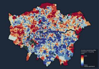
This visualisation shows a way of measuring affordability in London, comparing income with transport and housing costs.
There’s a story we all think we know about London and how expensive it is. The story is that people pay more on their housing in Central London whilst paying less in Outer London, which is somewhat offset by increased travel costs. Generally, that works out as Outer London being cheaper. These visualisations we created shows that this isn’t always the case by exploring the geographic patterns of travel and housing costs, as well as wage patterns. This is a really important story to tell, as a lot of people who live in London base some big life choices around this relationship.
What I enjoy about these visualisations is you can find your own story in them. London is such a complicated place that there are always about a million things that you can take away from any map of it. That’s one of this things I really love about geographic visualisations – you can hand someone your map or dashboard, and they can go and explore it themselves.
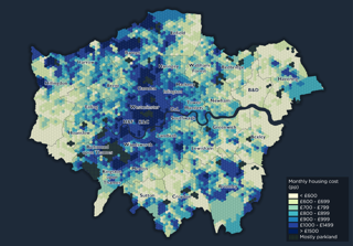
Monthly housing costs
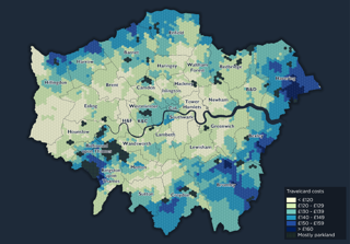
Travelcard costs
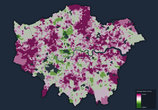
Average daily income
Why was it created?
Steer – the company I work for – joined up with Centre London Forward to do a research project about fair access to transport in Central London. I was given the initial question of ‘is there a relationship between deprivation and public transport accessibility?’ As with all research, this completely evolved – every bit of analysis threw up about 50 more questions that we wanted to explore. The research aimed to open people’s eyes to the reality of transport in London and see it as a more complex issue than simply inner London equals better transport links. We wanted policy makers, transport providers, developers and transport planners to move away from simplistic measures of travel-time accessibility when there are so many more factors at play.
Who was the intended audience?
Honestly, the original intended audience was a group of about seven London-based researchers and transport consultants. These visualisations were going to inform maybe a couple of bullets in a much bigger report. However as they grew and became a key element of that report, the audience changed. Our new audience of policy makers, transport providers and transport planners were still expertly familiar with London’s geography and were interested in the city as a whole, as opposed to local nuances, and because of this, we could dispose with a lot of geographic detail to allow for the data to tell its story.
This was a great exercise in how important ‘designing for your audience’ is. I posted these maps on Reddit and had lots of people wanting the opposite design – they wanted more geographic detail and zoomed in maps so they could identify what was going on where they specifically live.
What data did you use to create it and why?
There was a lot of different data that went into this! The UK – and particularly London – has some brilliant open data, and the main sources for this were TfL, the GLA, the Valuation Office Agency and of course the Census. We also did some bespoke public transport catchment journey time analysis using:
-
Average house price (Land Registry, 2018 or most recent)
-
Average social housing rent (Ministry of Housing, Communities and Local Government, 2018)
-
Average private housing rent (Valuation Office Agency, 2018)
-
Residents by tenure type (Census, 2011)
-
Monthly travel card prices and zones (TfL, 2019)
-
Location of usual residence and place of work by method of travel to work (Census,2011)
-
Average income (GLA)
-
Travel time to Central London (calculated by Steer)
Why did you choose to present the data in this way over other approaches?
We presented the data in a ‘hexcell’ format, which is a grid of interlocked hexagons. Most of the data we used came at census geography levels – if you aren’t familiar with these, they’re sized so that they all have a broadly similar population, and so have irregular shapes and sizes. Using a regular hexagonal geography to represent this data was useful as it stops the larger, but less densely populated, polygons dominating the visualisation while the smaller areas get lost. This also helps minimise any bias which stems from the creation of the census geography. Hexagons are particularly good for mapping for many reasons, including that they have a low area-to-perimeter ratio (which reduces sampling bias) and that they can represent geographic curves (e.g. patterns from roads or rail lines).
Then it was just about making the data engaging! I really like creating a bit of texture and depth in my maps, particularly when they’re ‘just’ choropleth maps. To do this I added a dark outer gradient to the London boundary to help the city stand out, and used a few layers of dark/light-to-transparent gradients to give a slightly bumpy effect (a few people have said this reminds them of a pin cushion). This is also a great and subtle way of distinguishing between discrete polygons without having to add a clunky line between them.
How have people engaged with the visualisation – what has it enabled people to do?
At Steer, having this ‘index’ of costs and affordability in London at our fingertips has been really useful for kickstarting projects as it gives us a good baseline understanding of the challenges and opportunities that an area might face.
From a personal perspective, going through some of this data has been incredibly eye opening. Did you know there’s an area north of Hampstead Heath where the average house price is 8 million pounds? I would have to work for 270 years to earn that much money! Everyone knows that inequality is a huge problem in London, but I think it’s hard to understand the scale of that without looking at the numbers. I think this work can help you confront what you think you know about London as a whole, but also about areas that you think you know and your own experiences of them.
How else might this approach or data be used? How can the visualisation be taken a step further?
I want to redo this in a post-covid world as I think what’s happening at the moment is really deepening the city’s inequality. As geographers I believe it’s our responsibility to really keep our collective foot down on analysing inequality, but also making sure people know about it. I also want to explore the travel card cost analysis – at the moment it’s based on residents travelling by all modes. I’d like to weight it by the modes they actually travel by, as I expect people living more centrally would be more inclined to walk, cycle or bus to work.
Try it yourself
All you need to recreate this is spreadsheet software and GIS which allows you to use transparent gradients (i.e. the ability to create a gradient from transparent to opaque – ArcPro, Adobe Illustrator and QGIS all have this functionality). The starting point for this was to aggregate all of the data outlined above to a single geography from which they can be combined and compared. This was done by creating a hexcell layer in QGIS (MMQGIS plugin) then allocating the data to each hexcell proportionally by area, using the intersect tool in ArcGIS/QGIS and then some simple modelling in excel to weight the data. As well as normalising the data by area, it also had to be normalised by unit to represent the same time period and person/household. One every hexcell had a value for each variable, looking at the relationships between them was straightforward.
About the creator
Helen McKenzie is a Senior Consultant at Steer Group, providing spatial analytics in the digital intelligence team, supporting company-wide GIS and map design needs.
Prior to joining Steer in 2016, she worked as a GIS consultant in the landscape design industry and has also worked in flood modelling and drone mapping.
You can find out more about Helen and her work on her Steer profile or by following her on Twitter @helenmakesmaps